Advanced Excel - Data Model

Advanced Microsoft Excel

Part 13 - Data Model

Excel 2013 has powerful data analysis features. You can build a data model, then create amazing interactive reports using Power View. You can also make use of the Microsoft Business Intelligence features and capabilities in Excel, PivotTables, Power Pivot, and Power View.

Data Model is used for building a model where data from various sources can be combined by creating relationships among the data sources. A Data Model integrates the tables, enabling extensive analysis using PivotTables, Power Pivot, and Power View.

A Data Model is created automatically when you import two or more tables simultaneously from a database. The existing database relationships between those tables is used to create the Data Model in Excel.

Step 1 − Open a new blank Workbook in Excel.

Step 2 − Click on the DATA tab.

Step 3 − In the Get External Data group, click on the option From Access. The Select Data Source dialog box opens.

Step 4 − Select Events.accdb, Events Access Database file.

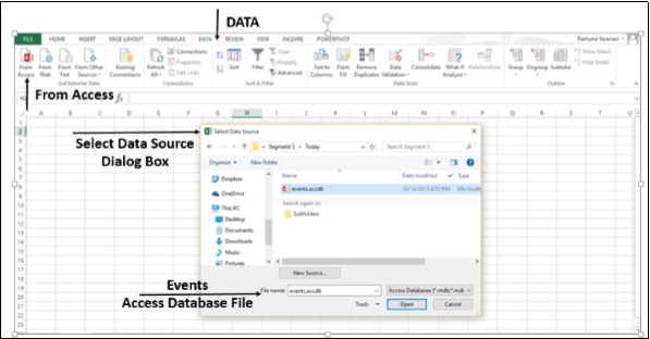
Step 5 − The Select Table window, displaying all the tables found in the database, appears.

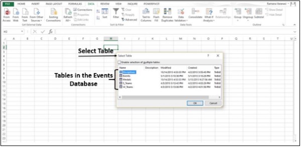
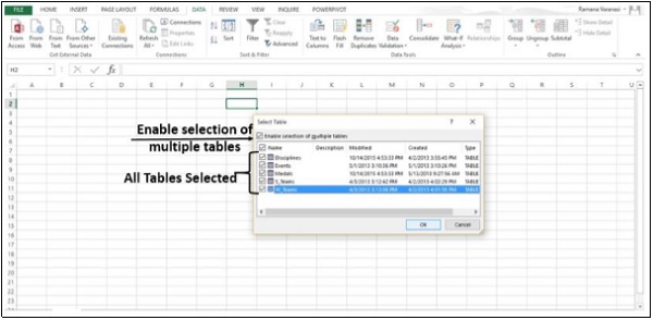
Step 6 − Tables in a database are similar to the tables in Excel. Check the ‘Enable selection of multiple tables’ box, and select all the tables. Then click OK.

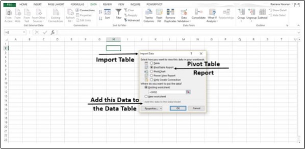
Step 7 − The Import Data window appears. Select the PivotTable Report option. This option imports the tables into Excel and prepares a PivotTable for analyzing the imported tables. Notice that the checkbox at the bottom of the window - ‘Add this data to the Data Model’ is selected and disabled.

Step 8 − The data is imported, and a PivotTable is created using the imported tables.

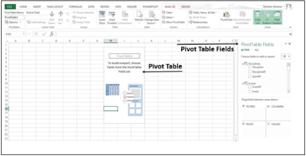
You have imported the data into Excel and the Data Model is created automatically. Now, you can explore data in the five tables, which have relationships defined among them.

Explore Data Using PivotTable

Step 1 − You know how to add fields to PivotTable and drag fields across areas. Even if you are not sure of the final report that you want, you can play with the data and choose the best-suited report.

In PivotTable Fields, click on the arrow beside the table - Medals to expand it to show the fields in that table. Drag the NOC_CountryRegion field in the Medals table to the COLUMNS area.

Step 2 − Drag Discipline from the Disciplines table to the ROWS area.

Step 3 − Filter Discipline to display only five sports: Archery, Diving, Fencing, Figure Skating, and Speed Skating. This can be done either in PivotTable Fields area, or from the Row Labels filter in the PivotTable itself.

Step 4 − In PivotTable Fields, from the Medals table, drag Medal to the VALUES area.

Step 5 − From the Medals table, select Medal again and drag it into the FILTERS area.

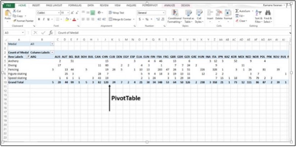
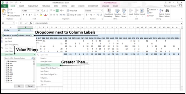
Step 6 − Click the dropdown list button to the right of the Column labels.

Step 7 − Select Value Filters and then select Greater Than…

Step 8 − Click OK.

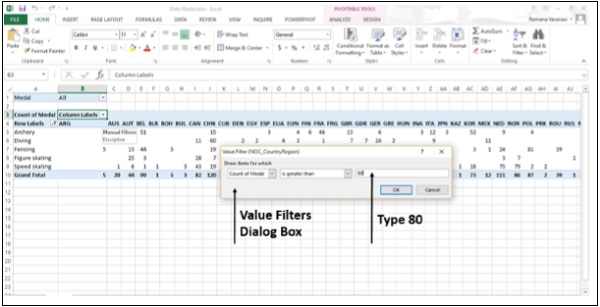
The Value Filters dialog box for the count of Medals is greater than appears.

Step 9 − Type 80 in the Right Field.

Step 10 − Click OK.

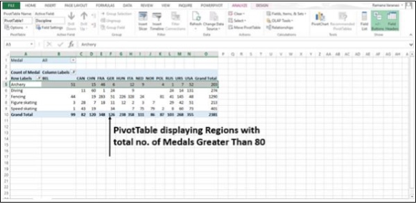
The PivotTable displays only those regions, which has more than total 80 medals.

You could analyze your data from the different tables and arrive at the specific report you want in just a few steps. This was possible because of the pre-existing relationships among the tables in the source database. As you imported all the tables from the database together at the same time, Excel recreated the relationships in its Data Model.

If you do not import the tables at the same time, or if the data is from different sources or if you add new tables to your Workbook, you have to create the Relationships among the Tables by yourself.

Create Relationship between Tables

Relationships let you analyze your collections of the data in Excel, and create interesting and aesthetic reports from the data you import.

Step 1 − Insert a new Worksheet.

Step 2 − Create a new table with new data. Name the new table as Sports.

Step 3 − Now you can create relationship between this new table and the other tables that already exist in the Data Model in Excel. Rename the Sheet1 as Medals and Sheet2 as Sports.

On the Medals sheet, in the PivotTable Fields List, click All. A complete list of available tables will be displayed. The newly added table - Sports will also be displayed.

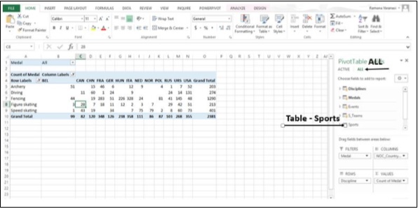
Step 4 − Click on Sports. In the expanded list of fields, select Sports. Excel messages you to create a relationship between tables.

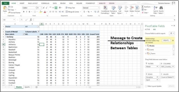
Step 5 − Click on CREATE. The Create Relationship dialog box opens.

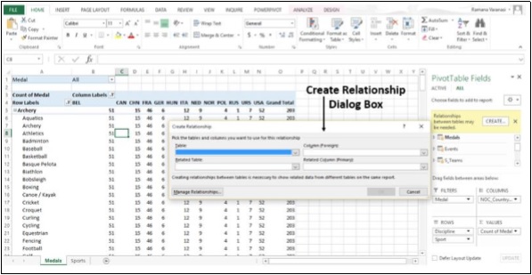
Step 6 − To create the relationship, one of the tables must have a column of unique, non-repeated, values. In the Disciplines table, SportID column has such values. The table Sports that we have created also has the SportID column. In Table, select Disciplines.

Step 7 − In Column (Foreign), select SportID.

Step 8 − In Related Table, select Sports.

Step 9 − In Related Column (Primary), SportID gets selected automatically. Click OK.

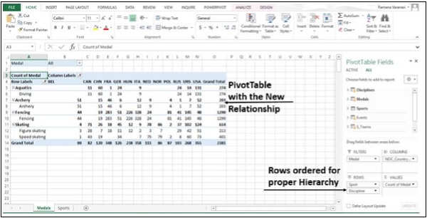
Step 10 − The PivotTable is modified to reflect the addition of the new Data Field Sport. Adjust the order of the fields in the Rows area to maintain the Hierarchy. In this case, Sport should be first and Discipline should be the next, as Discipline will be nested in Sport as a sub-category.