Advanced Excel - Discontinued Features

Advanced Microsoft Excel

Part 29 - Discontinued Features

Discontinued / Changed features

So far, you have seen the features that are added in Excel 2013. You also need to be aware of the −

• features existing in earlier versions of Excel that are no more available in Excel 2013, and
• the changed functionality in certain cases

Save Workspace

The Save Workspace command is no longer available in Excel. This command was used in earlier versions of Excel to save the current layout of all windows as a workspace. However, you can still open a workspace file (*.xlw) that was created in an earlier version of Excel.

New from Existing

In the earlier versions of Excel, the New from Existing option, which you get when you click File and then click New, let you base a new file on an existing one. This option is no longer available. Instead, you can open an existing Workbook and save it with a different file name.

• Step 1 − Click on File.
• Step 2 − Click on Save As. In the Save As dialog box give a different file name.

Alternatively, check if the workbook you want to use is in the Recent Workbooks folder.

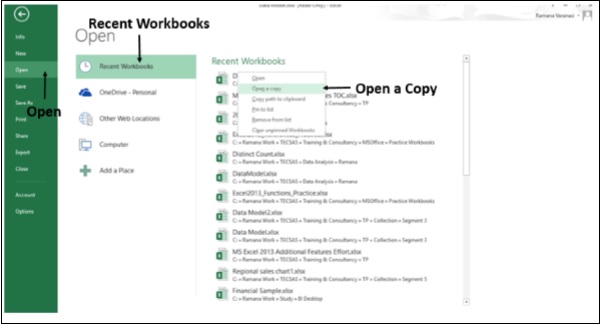
• Step 1 − Click on the File menu.
• Step 2 − Click on Open.
• Step 3 − Click on Recent Workbooks.

If the file is available there,

• Step 4 − Right-click on its file name.
• Step 5 − Then Click on Open a Copy.

Excel creates a copy of the file by adding a number to the file name. You can save the Workbook with a different file name as needed.

Save as Template

In the earlier versions of Excel, you can save a chart as a template on the Chart Tools ribbon by following the steps − Chart Tools → Design → Type.
In Excel 2013, Save as Template is no longer available on the Ribbon. To save a chart as a template −
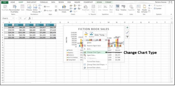
Step 1 − Right-click on the Chart.
Step 2 − Click on the Save as Template option.
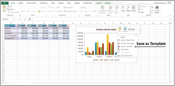Excel saves the chart as a Chart template (*.crtx) in the default Microsoft Templates folder.
You can use it to create a Chart or change a Chart Type.
Step 1 − Select a Data Table.
Step 2 − Click on the INSERT tab on the Ribbon.
Step 3 − Click on Recommended Charts in the Charts group.
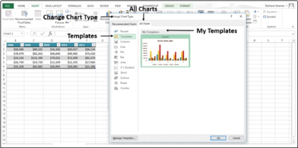
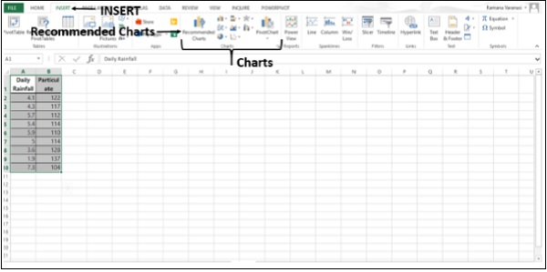The Insert chart window appears.
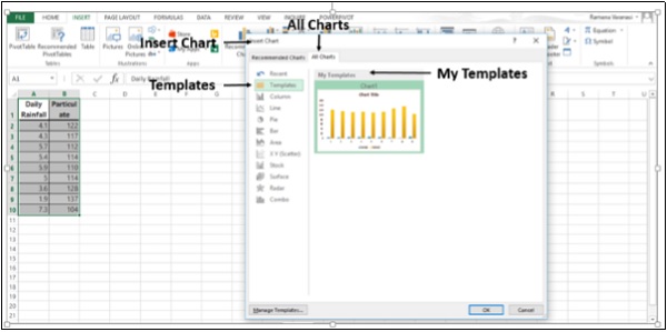
Step 4 − Click on the All Charts tab.
Step 5 − Click on Templates. Under the Header My Templates, your saved Chart Templates will be displayed.
Similarly, to change a Chart Type −
Step 1 − Right-click on a Chart.
Step 2 − Click on Change Chart Type.
The Change Chart Type window appears.
Step 3 − Click on the All Charts tab.
Step 4 − Click on Templates. Under the Header My Templates, your saved Chart Templates will be displayed.

Split Box Control

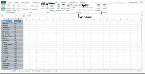
You used the Split Box Controls on the worksheet to split the window into panes at any position on the Worksheet in earlier versions of Excel. In Excel 2013, Split Box Control is removed.
Instead, you can use the Split Command on the ribbon.
Step 1 − Click on the VIEW tab on the Ribbon.
Step 2 − Select the cell where you want to place the Split. Click on Split in the Window Group.
The Split appears. As earlier, you can drag a split to reposition it, and double-click a split to remove it.

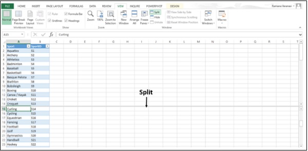
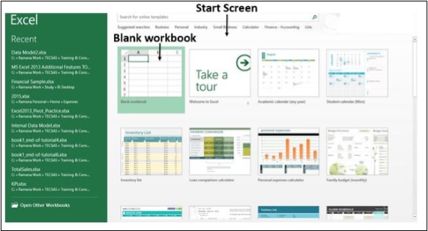
Blank Workbook

In the earlier versions of Excel, when you saved the Workbook settings, you frequently used a Workbook template called Book.xltx that is stored in the XLStart folder. This template would open automatically when you created a new blank Workbook.
When you start Excel 2013, the Start screen appears and Excel does not open a new Workbook automatically. The blank Workbook, which you click on the start screen is not associated with Book.xltx.
You can set up Excel to open a new Workbook automatically that uses Book.xltx −
Step 1 − Click on File.
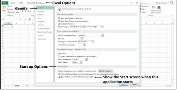
Step 2 − Click on Options. The Excel Options window appears.
Step 3 − Click on General.
Step 4 − Uncheck the Show the Start screen when this application starts box under the Start up options.
The next time you start Excel, it opens a Workbook that uses Book.xltx.

Save Options

In the earlier versions of Excel, when you saved a Workbook as a template, it automatically appeared in the My Templates folder under the Available Templates.
In Excel 2013, when you save a Workbook as a template, it will not automatically appear as a personal template on the new page.
Step 1 − Click on the File tab.
Step 2 − Click on Options.
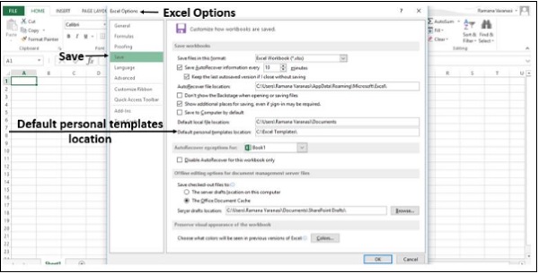
Step 3 − Click on Save.
In the default personal templates location box, enter the path to the templates folder you created.

Microsoft Clip Organizer

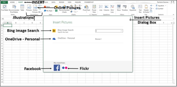
Microsoft Clip Organizer is no longer included in Office 2013. The Clip Organizer feature is replaced by the Insert Pictures dialog box (Insert > Online Pictures). This new Insert Online Pictures feature lets you find and insert content from the Office.com Clip Art collection and other online sources, such as Bing Image/Video search, Flickr, and your OneDrive or Facebook page.
In Excel 2013, Microsoft Clip Organizer is not included. Instead, you can insert Pictures from online sources such as Bing Image Search, Flickr, your OneDrive, and Facebook.
Step 1 − Click on the INSERT tab on the ribbon.
Step 2 − Click on the Online Pictures button in the Illustrations group. An Insert Pictures dialog box opens.
Step 3 − Select the picture from any of the sources.

MS Office Picture Manager

Microsoft Office Picture Manager is removed.

Exit option

In the earlier versions of Excel, you can exit Excel and close all the open workbooks at once. This was causing confusion among the different close and exit commands in Backstage View. Hence, it is removed.
Clicking on the File menu and then the Close option or the Close button (in the upper-right corner of the application window) closes the workbooks one at a time. If there are many open workbooks and you want to close all at once, it is time consuming because you can close only one workbook at a time.
If you want the Exit command available to you, you can add it to Quick Access Toolbar.
Step 1 − Click on the File tab.
Step 2 − Click on Options.
Step 3 − In the Excel Options window, click on the Quick Access Toolbar in the left pane. The option Customize the Quick Access Toolbar appears in the Right pane.
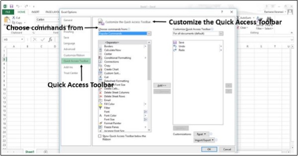Step 4 − In Choose commands from: select All Commands.
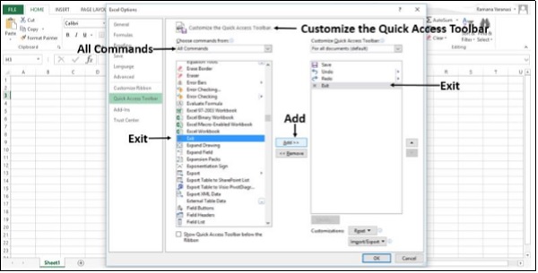
Step 5 − Select Exit.
Step 6 − Click on Add. The Exit command is added to the list on the right side.
Step 7 − Click on OK.
The Exit Excel Command appears on Quick Access Toolbar.
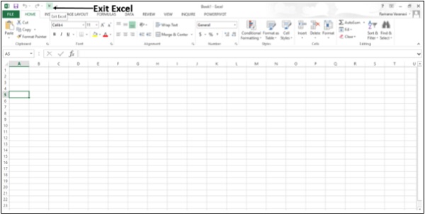Step 8 − Click on the Exit Excel command. All the open workbooks close at once.

Browser View Options

Earlier, when saving a workbook to the web, you used to set how users will see your workbook when they view it. These options used to be in the Save As dialog box when you saved a workbook to SharePoint.
In Excel 2013, first you need to set the Browser View options.
Step 1 − Click on File.
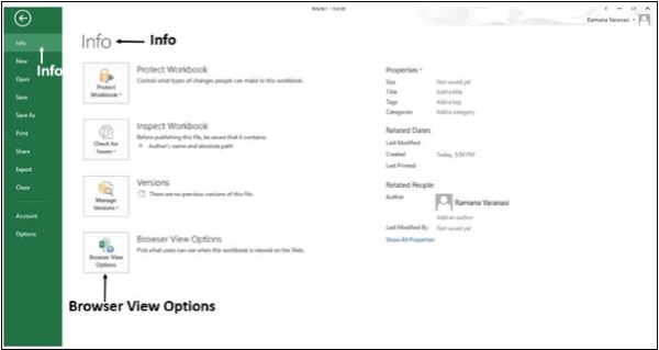
Step 2 − Click on Info.
Step 3 − In the Info pane, click on the Browser View Options.
Step 4 − In the Browser View Options window, select the options.
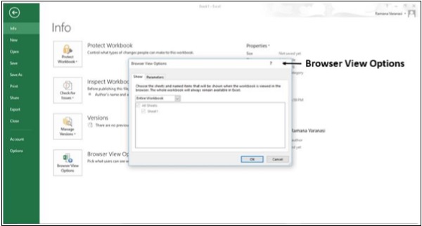Step 5 − Save the workbook to any web location.

Individual Data Series

In the earlier versions of Excel, you could change the Chart type of an individual data series to a different Chart type by selecting each series at a time. Excel would change the Chart type of the selected data series only.
In Excel 2013, Excel will automatically change the Chart type for all data series in the Chart.

Pyramid and Cone Chart Types

The Column and Bar Charts are removed from the Pyramid and Cone Chart types in the Insert Chart and Change Chart Type dialog boxes.
However, you can apply Pyramid and Cone shapes to any 3-D Column or Bar Chart.
Step 1 − Right-click on the 3-D Column chart.
Step 2 − Click on Format Data Series.
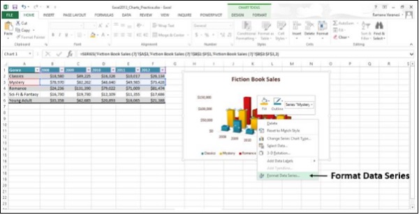Step 3 − Select the shape you want.
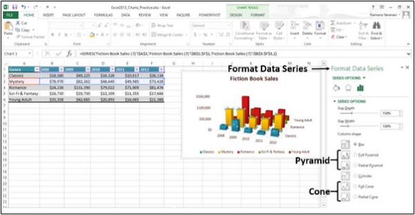The required format will be displayed.

---